Map Builder

A map in GeoLens is a saved composition: a stack of layers, each with its own data source, style rules, and filter expression, plus a viewport (center, zoom, and basemap) that determines what you see when the map first loads. Maps are first-class catalog citizens — they’re searchable, taggable, and shareable, and they re-render against live data so the underlying layers stay current.

This page walks through how to build a map: starting fresh, adding layers, styling them, filtering, optional AI-assisted composition, and sharing.

Creating a map

There are two ways to create a map:

Start blank — from the Maps section in the sidebar, click New map. You’ll land on an empty canvas with the default basemap.
Start from a dataset — from any dataset detail page, click Add to map. GeoLens creates a new map with that dataset as the first layer, opens the Map Builder, and zooms to the dataset’s extent.

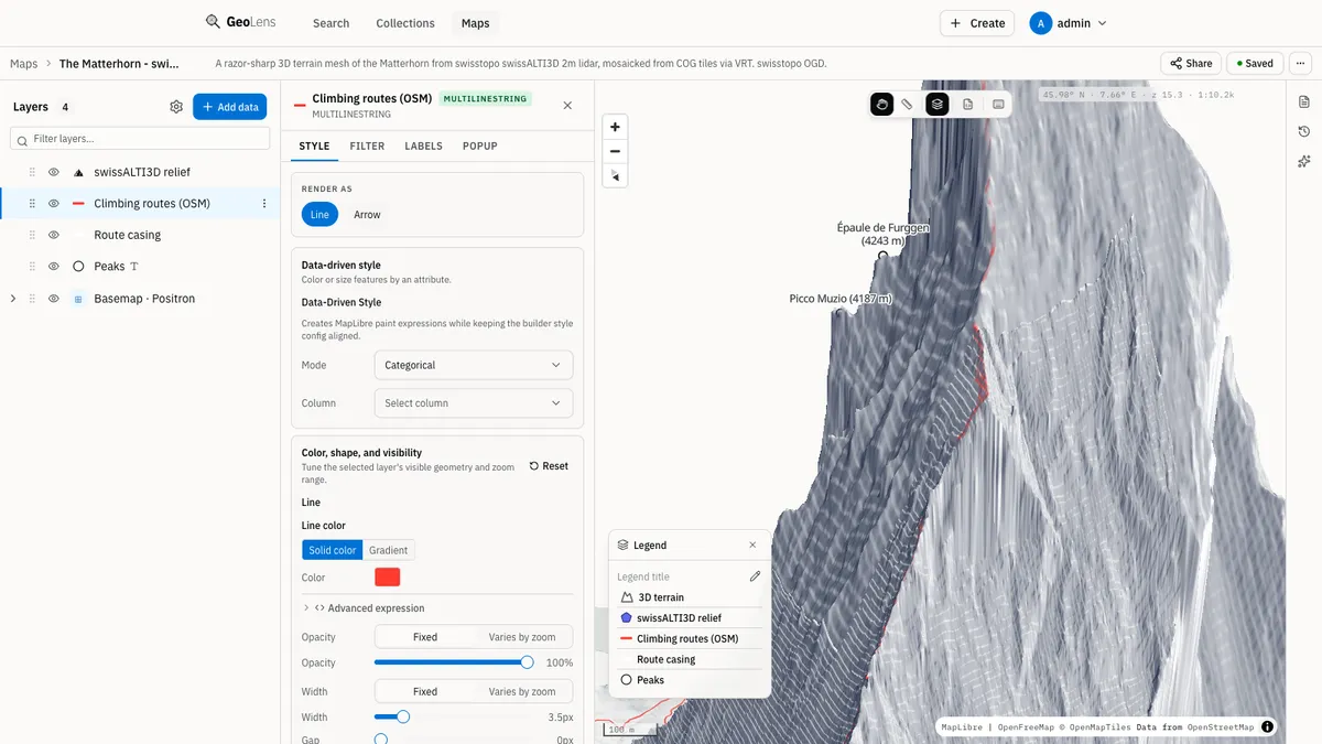
The canvas has three main regions:

Layer panel (left) — the list of layers, with reorder handles, per-layer visibility toggles, and per-layer settings (style, filter, source).
Map canvas (center) — the actual map view; zoom and pan with mouse, pinch-zoom on touch.
Inspector (right) — context-sensitive panel that opens when you select a layer, click a feature, or open the AI chat. By default it’s collapsed.

The map auto-saves as you work; there’s no separate Save button for basic edits. Adding/removing layers, updating styles, and changing the viewport all persist immediately.

Layers

A layer is one dataset rendered on the map with a specific style and optional filter. Most maps have between 1 and 10 layers; there’s no hard upper bound, but very dense compositions slow rendering.

Layer types

GeoLens supports several layer types, depending on the source dataset:

Vector — points, lines, or polygons rendered client-side from MVT tiles. The default for vector datasets in your catalog.
Raster — image tiles served from titiler with on-the-fly band expressions, colormaps, and rescaling. The default for raster datasets.
WMS — external Web Map Service. Useful for inline-rendering an external basemap, an external thematic layer, or a competing-platform service you’ve registered.
WFS / OGC API Features — external vector service. Pulls vector features from a registered service URL at view time.
Imported file — a one-off layer from a Shapefile/GeoJSON/GeoPackage uploaded directly into the Map Builder rather than the catalog. Useful for ad-hoc overlays you don’t want to persist as a catalog dataset.

For external services (WMS, WFS, OGC API), the URL is registered through Importing Data and reused across maps; you don’t paste a URL into the Map Builder directly.

Adding and reordering layers

Click Add layer at the top of the layer panel to open the layer picker. The picker shows your catalog with the same search experience as Search & Discovery — keyword, tags, geometry type, bbox. Select a dataset (or several with shift-click) and click Add to push them onto the layer stack.

Drag the handle on a layer’s row in the layer panel to reorder. Layers render top-down: the topmost layer in the panel renders on top of the canvas. A common pattern is to put base data (population, terrain) at the bottom and overlays (boundaries, points of interest) at the top.

Toggling visibility and removing

Each layer has an eye icon to toggle visibility without removing it (useful while comparing alternatives) and a kebab menu with Duplicate, Edit source, and Remove.

Styling

Each layer has its own style. Open a layer’s row in the panel and click the Style tab in the inspector to edit.

Vector styling

Vector layers expose three style families:

Point — circle, symbol (icon), or text. Configure radius, color, outline, and per-attribute styling.
Line — color, width, dash pattern, line-join behavior.
Fill — color, opacity, outline color, outline width.

For each, you can set a single static value (e.g., “all points red, radius 4 pixels”) or drive the value from an attribute:

Categorical — different color per unique value of an attribute (e.g., one color per land_use category).
Continuous (color ramp) — interpolate a color ramp across a numeric attribute (e.g., choropleth on population_density).
Step — discrete bins with explicit thresholds (e.g., “below 100 = green, 100-500 = yellow, above 500 = red”).

Color ramps include the standard scientific options (viridis, plasma, magma, inferno, cividis), plus diverging ramps (RdBu, BrBG) and sequential ramps (Blues, Greens, Purples).

Raster styling

Raster layers expose:

Band selection — for multi-band rasters, pick one band (single-band rendering with a colormap) or three bands (RGB rendering, e.g., from a satellite image).
Rescaling — clip the input range to a min/max for each band; values outside are clamped.
Colormap — for single-band rendering, pick from the same scientific ramps available for vector continuous styling.
Resampling — nearest, bilinear, or cubic; nearest preserves categorical-raster pixel boundaries, bilinear/cubic smooth continuous rasters.

Filters

A layer filter is a CQL2 expression evaluated server-side; only features matching the expression are rendered. Filters reduce visual clutter and improve performance on dense layers.

Common filter patterns:

Equality — land_use = 'residential'
Comparison — population > 10000
Range — year >= 2020 AND year <= 2024
Set membership — state IN ('CA', 'OR', 'WA')
Spatial — INTERSECTS(geom, BBOX(-122.5, 37.5, -122.0, 38.0))
Combined — population > 10000 AND state = 'CA'

The filter input has syntax highlighting and validates on each keystroke; errors appear inline. The filter is also applied to the layer’s bbox, so zooming auto-fits to the filtered subset.

For the full CQL2 grammar and the API equivalents, see OGC API & Standards Endpoints — the same expressions work in ?filter= query parameters on /api/collections/{id}/items.

AI chat (admin-configurable)

If your administrator has enabled AI features for your instance, an AI chat panel appears in the inspector. The AI assistant helps with map composition tasks:

Suggesting CQL2 filter expressions from natural language (“show only populated places with more than 50,000 people in California”).
Suggesting styles based on attribute distributions (“style this dataset as a choropleth on gdp_per_capita”).
Answering questions about layer data (“what’s the highest population value in this layer?”).
Recommending layer order or style refinements based on the visible map.

The AI chat is scoped to map composition — it doesn’t navigate the catalog on your behalf, ingest new data, or modify metadata. Its context is your current map state, the active layers, and the schema/sample of attributes in those layers.

Maps have three sharing modes, set from the Share button in the page header.

Private — only you (and admins) can open this map. Useful for drafts.
Public — anyone with the URL can open the map. The map renders read-only for non-logged-in viewers — they can’t edit, but they can pan, zoom, and click features.
Restricted — explicit list of users or groups with access, similar to dataset visibility (see the Access tab on the dataset detail page).

The share URL is the same as the map’s edit URL but with ?embed=1 for the embed variant — a chrome-free version suitable for an iframe.

Embed iframe

The Share dialog generates an embed snippet:

<iframe
  src="https://your-instance/maps/<map-id>?embed=1"
  width="100%"
  height="600"
  frameborder="0"
></iframe>

The embed strips the GeoLens header/sidebar and renders the map full-bleed. It honors the same access controls as the regular share URL — viewers must have permission to see all layers in the map.

Permission scope

The map’s visibility cascades to its layers: a public map’s layers must all be public datasets, or the layer is silently hidden for unauthenticated viewers. The Share dialog flags any layers that won’t render for the intended audience and offers to either change the dataset visibility or remove the layer.

Tips

Use saved searches as filter starting points. A saved search in Search & Discovery captures a CQL2-equivalent filter; you can copy the expression and paste it into a layer’s filter to render the same subset on a map.
Layer ordering matters for performance. Heavy raster layers at the top of the stack force the renderer to do more work even if vector layers above are fully transparent. Put background rasters at the bottom.
Duplicate before experimenting. Use the Duplicate option on a layer to preserve the original style while you try something new.
Use bbox filtering at view zoom. A layer with BBOX(...) filter scoped to your typical viewport renders much faster than the same layer unfiltered — especially for dense polygon datasets.